On Getting Confidence Estimates from Neural Networks
I've been reading on and off about this topic for a while now, and it comes up very often in applied ML. How confident is the neural network about a particular prediction it makes? Can we switch to a different end user experience when the network is not confident? In a typical scenario, a model is trained on a limited dataset and gets deployed in a product, where unless the user experience is strictly guarded, the model will get hit with inputs that were not anticipated. This is the problem of Out-Of-Distribution (OOD) detection - and if a model can either say that it does not "know" what to do in such cases, or equivalently, make a low confidence prediction - then that is useful for avoiding catastrophic failures.
There is a lot of research that focuses on this topic, and what follows is a summary of some of the papers I've read.
Measuring Confidence
So how do we measure the confidence of a neural network? The majority of research focuses on Classification models, so we'll talk about them first, with a section on regression models at the end.
Classification models
Classification models output the probability of a sample belonging to a given class, and intuitively, the probability estimate should itself be a measure of confidence. That is, we could say that max(softmax_scores) is a measure of confidence. And then, for OOD detection, we say that a sample is OOD if max(softmax_scores) < threshold
inputs = np.random.randn(42)
softmax_scores = model(inputs)
predicted_class = np.argmax(softmax_scores)
confidence = np.max(softmax_scores)
print("I say Class {:d} with {:.2f} confidence".format(predicted_class, confidence))
I say Class 1 with 0.58 confidence
Is this a good measure of confidence?
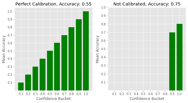
Yes, if the model is well calibrated. A model's calibration is typically understood via Reliability Diagrams, where we plot binned confidence estimates on the x-axis and model accuracy on the y-axis. For a perfectly calibrated model, 90% of the samples that have a confidence score of 0.9 would be correctly classified. So, when we plot accuracy against confidence, we should see a nice line along the diagonal for a perfectly calibrated model.
On the other hand, as noted in On Calibration of Modern Neural Networks, max(softmax_scores) for modern neural networks skew higher, and thus the models are not well calibrated, even though they achieve higher accuracy overall.
plot_sample_reliability_diagrams()
Why does this happen?
The first question that comes to mind - Why do modern neural nets behave this way? Unfortunately, there is no definitive answer to this question, but the authors in [1] have some results that indicate a relation to overfitting and model capacity. Specifically, calibration error increases with the number of model parameters, and also as weight decay is reduced. It seems like the same phenomenon that leads to failure modes such as adversarial errors is at play here, and techniques that make a model more robust also help with calibration and OOD detection.
What can be done?
Temperature Scaling
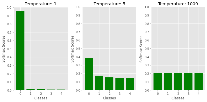
This is the simplest method, and has been found to be effective in [1], [2] and [3]. Scale the logits with a temperature parameter T to obtain modified softmax scores, and then use max(softmax_scores) as before. Optimal value of T is typically chosen via hyperparameter search on a validation set - but in general, a value > 1 makes sense. As T increases, the output distribution entropy increases - so for T > 1, the output predictions become smoother, thus suppressing overconfident predictions and improving calibration. The authors in [2] show that this effect is more pronounced for OOD samples than for in-distribution ones, which leads to gains in OOD detection as well.
scores = np.exp(logits / T) / np.sum(np.exp(logits / T))
demo_temperature_scaling()
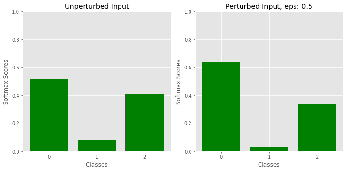
Input perturbation
This method, proposed in [2] is similar in principle to methods such as FGSM used for generating adversarial samples. Given an input x, we generate a modified input x' by moving in the direction of the gradient that increases the score for the top scoring class. Note that this is the reverse of adversarial perturbation, where the input is jittered so as to produce a misclassification. The authors in [2] propose this technique for OOD detection - with the reasoning that the gradients are larger for in-distribution samples than OOD, thus increasing the margin of separation between the two. The effects of this technique on model calibration is unclear - but it is likely to make a model even less calibrated than before.
scores = model(x)
max_score = max(scores)
derivative = d/dx (max_score)
x' = x + epsilon * derivative
scores' = model(x')
demo_input_perturbation()
Model Ensembles
Model ensembles can be used to obtain a measure of uncertainty in the model predictions. The authors in [8] train multiple models with different random initializations and random shuffling of input data. Test time random dropout could also be used as a form of ensembling if re-training is not an option.
Mahalanobis Distance Measure in Feature Space
Given a pre-trained neural network, the authors in [3] propose an alternate measure of confidence based on the Mahalanobis distance. Class conditioned Gaussian distributions D_1, D_2, ... D_c with a shared covariance matrix are fit on the features from the penultimate layer of the network. During inference, we forward prop the sample x to obtain features f(x), and then use the Mahalanobis distance of f(x) from the closest distribution D_c' as our confidence measure. Note that the class prediction for sample x would be c', since that's the closest distribution.
Given c classes, and training data D:
Fit means µ_1, µ_2 ... µ_c and covariance Σ on features from D

Given new sample x:

conf_measure = -np.inf
for c in range(num_classes):
    features_x = model(x)
    dist_c = mahalanobis_distance(µ_c, Σ, features_x)
    conf_measure = max(conf_measure, -dist_c)
This follows from the general intuition that if we have a good generative model P(x) for our data, then OOD detection should be easy, because P(x) would be low for OOD samples. Since building a good generative model for images is hard, and even then, generative models on images such as PixelCNN++ have been shown to suffer from the same problem - lack of robustness to OOD samples [12]. So then, could we instead fit a generative model in the feature space of a pre-trained neural network? Since the model is trained for classification, it follows that a class conditional Gaussian distribution is a reasonable choice for the penultimate layer features.
Learned Confidence
Why not just have the model output its confidence in addition to the classification probability? How would we train such a head? This was explored in [4], and is rather neat. Given the model class predictions p and a confidence prediction c, they modify the prediction so:
Given data (x, y):
    p, c = model(x)
    p' = c * p + (1 - c) * y
    l_xent = xent(p', y)
where y is the actual label for the data point x. That is, if the model is confident, then it keeps its prediction p, and if it is not, then it gets to peak at the label y. With the cross entropy loss, this means that the model has two ways to drive the loss down: (a) make a confident correct prediction or (b) say that it is not confident by outputting a low c. This is what we want, but a trivial solution is to predict c = 0 for everything, so to prevent that, the authors add a second loss term like so:
l_conf = log(c)
l_total = l_xent + l_conf
During inference, the confidence prediction c can be thresholded to make OOD detections.
Outlier Exposure
This method, introduced in [5], provides a framework to introduce auxiliary data into the model training process to improve OOD/outlier detection. This is great if you can re-train your models, and have access to auxiliary datasets. In addition to the standard cross entropy loss on the labeled training dataset (considered in-distribution), we now have a different loss function on the unlabeled auxiliary dataset that can take different forms - the most common one being just the cross entropy between the model output and the uniform distribution over classes.
Even when there aren't additional data sources available, synthetically generating new ones, via adversarial perturbation, for example, has been found to be effective.
Given labeled data (x_i, y_i) and auxiliary data (x_j):

l_labeled = xent(model(x_i), y_i)
l_auxiliary = xent(model(x_j), uniform_over_classes)
l_total = l_labeled + lambda * l_auxiliary
This method can be combined with the Learned Confidence method above by training the network to predict c = 0 for the auxiliary dataset.
Energy based models
A recent paper on this topic [6] proposes a confidence score based on the Energy based Model interpretation of classification networks [7]. The idea is that the logits from a classification network can be reinterpreted to define energy scores as follows:
logits = model(x)
E(x, y) = -logits[y]
p(x, y) = exp(-E(x, y)) / Z, where Z is the normalizing constant

p(x) = sum_over_y(exp(-E(x, y))) / Z
p(x) = sum_over_y(exp(logits[y])) / Z

log(p(x)) = LogSumExp(logits) - Log(z)
The normalizing constant Z is intractable, but the authors make the observation in [6] that it is a constant, and hence, for the purposes of OOD detection, we can simply compare LogSumExp(logits). For in-distribution samples, we expect log(p(x)), and hence LogSumExp(logits) to be higher, and conversely, for OOD samples, LogSumExp(logits) should be lower. Thus, we define a confidence score as follows:
conf_score = LogSumExp(logits)
and then threshold this score for OOD detection. This metric can be used as is on a pre-trained network and is found to be superior to using max(softmax_score). More interesting is the case when the model can be re-trained explicitly so that LogSumExp(logits) is higher for in distribution samples than for OOD. In essence, we are training a generative model p(x) in addition to the conditional model p(y|x), and [7] goes into a lot of interesting detail on this. For OOD detection however, the authors in [6] propose a simpler loss function that enforces a margin of separation between in-distribution and OOD data from an auxiliary dataset. The problem framework is similar to Outlier Exposure, in the sense than an auxiliary dataset is considered available, and a loss function is defined on this data that helps with OOD / calibration.
l_labeled = xent(model(x_i), y_i) + np.square(max(0, -LogSumExp(logits) - margin_in))
l_auxiliary = np.square(max(0, margin_out + LogSumExp(logits)))
l_total = l_labeled + l_auxiliary
Regression Models
Learned Variance
Similar to Learned-Confidence, the authors in [8] set up a neural network that predicts both the mean µ and variance σ of the target variable. With the assumption that p(y|x) follows a Gaussian distribution with mean µ_x and variance σ_x, both predicted by the network, we train the model by minimizing the log likelihood.
µ, σ = model(x)
p(y|x) ∝ (1/σ) * exp(-1/2 * np.square((y -  µ)/σ))
log(p(y|x)) ∝ -log(σ) - (-1/2 * np.square((y -  µ)/σ))
The authors show that the learned σ is superior to empirical variance calculated using model ensembles as far as calibration is concerned. Appendix section A2 from [8] is intereseting, as it also outlines the method for calculating reliability diagrams for regression models.
References
- On Calibration of Modern Neural Networks
- Enhancing the Reliability of Out Of Distribution Image Detection in Neural Networks
- A Simple Unified Framework for Detecting Out-of-Distribution Samples and Adversarial Attacks
- Learning Confidence for Out-of-Distribution Detection in Neural Networks
- Deep Anomaly Detection with Outlier Exposure
- Energy based models for Out Of Distribution Detection
- Your Classifier is Secretly an Energy Based Model and You Should Treat it Like One
- Simple and Scalable Predictive Uncertainty Estimation using Deep Ensembles
- NeurIPS 2020 - Practical Uncertainty Estimation & Out-of-Distribution Robustness in Deep Learning
- Likelihood Ratios for Out-of-Distribution Detection
- Dropout as a Bayesian Approximation: Representing Model Uncertainty in Deep Learning
- Do deep generative models know what they don’t know?
import numpy as np
from matplotlib import pyplot as plt

%matplotlib inline

def model(inputs):
    logits = np.random.randn(5) # 5 classes
    return np.exp(logits) / np.sum(np.exp(logits))

def demo_input_perturbation():
    def get_scores(x):
        logits = np.array([x*x, 1 - x*x, x])
        scores = np.exp(logits) / np.sum(np.exp(logits))
        return scores
    def get_derivative(x):
        return np.exp(x*x) * (4 * x * np.exp(1 - x*x) + (2*x - 1)*(np.exp(x))) / np.square((np.exp(x*x) + np.exp(1 - x*x) + np.exp(x)))

    x = 1.2
    scores = get_scores(x)
    derivative = get_derivative(x)
    eps = 0.5
    x_dash = x + eps * derivative
    scores_dash = get_scores(x_dash)
    _, ax = plt.subplots(1, 2, figsize=(10, 5))
    ax[0].bar(range(3), scores, color='green')
    ax[0].set_title("Unperturbed Input")

    ax[1].bar(range(3), scores_dash, color='green')
    ax[1].set_title("Perturbed Input, eps: 0.5")

    for ax_indx in [0, 1]:
        ax[ax_indx].set_ylim((0.0, 1.0))
        ax[ax_indx].set_xticks(range(3))
        ax[ax_indx].set_xticklabels(range(3))
        ax[ax_indx].set_xticks(range(3))
        ax[ax_indx].set_xticklabels(range(3))
        ax[ax_indx].set_xlabel('Classes')
        ax[ax_indx].set_ylabel('Softmax Scores')
    plt.tight_layout()
    plt.show()


def demo_temperature_scaling():
    logits = np.array([5, 1, 0.3, 0.1, 0.1])
    yticks = [0, 0.1, 0.2, 0.3, 0.4, 0.5, 0.6, 0.7, 0.8, 0.9, 1.0]
    ts = [1, 5, 1000]
    _, ax = plt.subplots(1, len(ts), figsize=(10, 5))
    for indx in range(3):
        mod_logits = logits / ts[indx]
        scores = np.exp(mod_logits) / np.sum(np.exp(mod_logits))
        ax[indx].bar(range(5), scores, color='green')
        ax[indx].set_title("Temperature: {}".format(ts[indx]))
        ax[indx].set_yticks(yticks)
        ax[indx].set_ylabel('Softmax Scores')
        ax[indx].set_xlabel('Classes')
        ax[indx].set_xticks(range(5))
        ax[indx].set_xticklabels(range(5))
    plt.tight_layout()
    plt.show()

def plot_sample_reliability_diagrams():
    plt.style.use('ggplot')
    _, ax = plt.subplots(1, 2, figsize=(10,5))

    confidence_xbar = np.array([0.1, 0.2, 0.3, 0.4, 0.5, 0.6, 0.7, 0.8, 0.9, 1.0])
    accuracy_ybar = np.array([0.1, 0.2, 0.3, 0.4, 0.5, 0.6, 0.7, 0.8, 0.9, 1.0])

    is_correct = np.zeros((10, 10))
    for i in range(10):
        is_correct[i, :(i+1)] = 1
    ax[0].bar([i for i,_ in enumerate(confidence_xbar)], np.mean(is_correct, axis=-1), color='green')
    overall_accuracy = np.mean(is_correct)
    ax[0].set_title("Perfect Calibration, Accuracy: {:.2f}".format(overall_accuracy))

    # What if we were very confident about all our predictions
    confidences = np.concatenate([np.ones((5, 10)) * 0.9, np.ones((5, 10)) * 1.0], axis=0)
    is_correct = np.zeros((2,10))
    is_correct[0, :7] = 1
    is_correct[1, :8] = 1
    overall_accuracy = np.mean(is_correct)
    ax[1].bar([i for i,_ in enumerate(confidence_xbar)], np.concatenate([np.zeros((8,)), np.mean(is_correct, axis=-1)], axis=0), color='green')
    ax[1].set_title("Not Calibrated, Accuracy: {:.2f}".format(overall_accuracy))

    for ax_indx in [0, 1]:
        ax[ax_indx].set_xlabel("Confidence Bucket")
        ax[ax_indx].set_ylabel("Mean Accuracy")
        ax[ax_indx].set_xticks(range(10))
        ax[ax_indx].set_xticklabels(confidence_xbar)
        ax[ax_indx].set_yticks(accuracy_ybar)
        ax[ax_indx].set_yticklabels(accuracy_ybar)

    plt.show()